
| Star | Watch | Fork |
| Home |
|---|
| User Guide |
| Examples |
| About |
Mean-Risk Portfolio Optimization with a Wasserstein Ambiguity Set
In this example, we consider the mean-risk portfolio optimization problem discussed in the paper Mohajerin Esfahani and Kuhn (2018). Assume that in a capital market consisting of \(m\) assets whose yearly returns are captured by the random vector \(\pmb{z} = (z_1, …, z_m)\), the investor is making a decision \(\pmb{x} = (x_1, … x_m)\), where each \(x_i\) indicates the percentage of the available capital invested in the \(i\)th asset. The portfolio optimization problem is formulated as the following distributionally robust model,
\[\begin{align} \min~&\sup\limits_{\mathbb{P}\in\mathcal{F}(\epsilon)} \mathbb{E}_{\mathbb{P}} \left[-\pmb{z}^{\top}\pmb{x} + \rho\left(\tau + \frac{1}{\alpha}\max\left\{-\pmb{z}^{\top}\pmb{x} - \tau, 0\right\}\right)\right] \\ \text{s.t.} ~&\pmb{1}^{\top}\pmb{x} = 1 \\ &\pmb{x}\in\mathbb{R}_+^m, \end{align}\]where the objective is to a weighted summation of the mean and the conditional value at risk (CVaR) of the portfolio loss \(-\pmb{z}^{\top}\pmb{x}\). The constant \(\alpha \in (0, 1]\) is referred to as the confidence level of the CVaR, and \(\rho \in \mathbb{R}_{+}\) quantifies the investor’s risk-aversion. The objective function can be replaced by the equivalent expression introduced in Rockafellar and Uryasev (2000), so the model above can be rewritten as follows,
\[\begin{align} \min~&\sup\limits_{\mathbb{P}\in\mathcal{F}(\epsilon)} \mathbb{E}_{\mathbb{P}} \left[\max\limits_{k\leq K} \left\{a_k \pmb{z}^{\top} \pmb{x} + b_k \tau\right\}\right] \\ \text{s.t.} ~&\pmb{1}^{\top}\pmb{x} = 1 \\ &\pmb{x}\in\mathbb{R}_+^m, \end{align}\]where \(K=2\), and coefficients \(a_k\) and \(b_k\) of the piecewise linear function are given below.
\[\begin{cases} a_1 = -1,~& b_1 = \rho \\ a_2 = -1 - \frac{\rho}{\alpha}, ~& b_2 = \rho(1-\frac{1}{\alpha}). \end{cases}\]Lastly, the set \(\mathcal{F}(\epsilon)\) of distributions is a Wasserstein ambiguity set with the radius to be \(\epsilon\). According to Chen et al. (2020), such an ambiguity set can be written as the following expression,
\[\begin{align} \mathcal{F}(\epsilon) = \left\{ \mathbb{P} \in \mathcal{P}_0\left(\mathbb{R}^m\times\mathbb{R}\times [n]\right)~ \left| ~\begin{array}{ll} (\tilde{\pmb{z}}, \tilde{u}, \tilde{j}) \in \mathbb{P} &\\ \mathbb{E}_{\mathbb{P}}\left[\tilde{u}\right] \leq \epsilon & \\ \mathbb{P}\left[\left.(\pmb{z}, u)\in\mathcal{Z}_{j} ~\right| \tilde{j} = j\right] = 1 & \forall j \in [n] \\ \mathbb{P}\left[\tilde{j} = j\right] = \frac{1}{n} & \end{array} \right. \right\}, \end{align}\]where \(n\) is the number of records in the historical data of the yearly return \(\pmb{z}\), and the support \(\mathcal{Z}_j = \left\{(\pmb{z}, u):~|\pmb{z} - \hat{\pmb{z}}_j |_1 \leq u, ~ \pmb{z} \geq -\pmb{1} \right\}\) captures the one-norm centered at the historical record \(\hat{\pmb{z}}_j\).
Following the paper Mohajerin Esfahani and Kuhn (2018), model parameters are summarized as below:
- Sample size of the empirical dataset \(n=30\);
- Number of assets \(m=10\);
- The empirical dataset \(\hat{\pmb{z}}\) used to represent the distribution of the random return \(z_i = \varphi + \zeta_i\), where \(\varphi \sim \mathcal{N}(0, 2\%)\) and \(\zeta_i \sim \mathcal{N}(i\times 3\%, i\times 2.5\%)\);
- The risk-aversion coefficient \(\rho=10\);
- The confidence level \(1-\alpha=80\%\);
- Wasserstein ball radius \(\epsilon=0.01\);
and these parameters are defined by the following code segment.
import numpy as np

n, m = 30, 10
i = np.arange(1, m+1)
np.random.seed(1)
phi = 0.02 * np.random.normal(size=(n, m))
zeta = 0.03*i + 0.025*i*np.random.normal(size=(n, m))
zhat = np.maximum(phi + zeta, -1)         # historical data of yearly return

epsilon = 1e-2                            # radius of the Wasserstein ball
rho = 10                                  # risk-aversion coefficient
alpha = 0.2                               # confidence level

a1, b1 = -1, rho                          # coefficients of the piecewise expression
a2, b2 = -1 - rho/alpha, rho - rho/alpha  # coefficients of the piecewise expression
Deterministic Equivalent Problem
According to Corollary 5.1 of Mohajerin Esfahani and Kuhn (2018), the distributionally robust model above is equivalent to deterministic problem,
\[\begin{align} \min ~&\lambda \epsilon + \frac{1}{n}\sum\limits_{i=1}^n s_i \\ \text{s.t.} ~&\sum\limits_{i=1}^m x_i = 1 & \\ &x_i \geq 0, &\forall i \in [m] \\ &b_k \tau + a_k \hat{\pmb{z}}_j^{\top}\pmb{x} + \pmb{\gamma}_{jk}^{\top}(\pmb{d} - \pmb{C}\hat{\pmb{z}}_j) \leq s_j &\forall j \in [n], \forall k \in [K] \\ &\|\pmb{C}^{\top}\pmb{\gamma}_{jk} - a_k\pmb{x}\|_{\infty} \leq \lambda \\ &\pmb{\gamma}_{jk} \in \mathbb{R}_{+}^{m} & \forall j \in [n], \forall k \in [K] \end{align}\]where the matrix \(\pmb{C} = -\pmb{I}\), and the vector \(\pmb{d} = \pmb{1}\), as a result of the support constraint \(\pmb{z} \geq -\pmb{1}\). The deterministic problem is solved using the code below.
from rsome import ro
import rsome as rso

C = - np.eye(m)
d = np.ones(m)

model = ro.Model()

x = model.dvar(m)
lamb = model.dvar()
gamma = model.dvar((2, n, m))
tau = model.dvar()
s = model.dvar(n)

model.min(lamb*epsilon + (1/n)*s.sum())
model.st(x.sum() == 1, x >= 0)
model.st(b1*tau + a1*(zhat@x) + (gamma[0]*(1 + zhat)).sum(axis=1) <= s)
model.st(b2*tau + a2*(zhat@x) + (gamma[1]*(1 + zhat)).sum(axis=1) <= s)
for i in range(n):
    model.st(rso.norm(-gamma[0, i] - a1*x, 'inf') <= lamb)
    model.st(rso.norm(-gamma[1, i] - a2*x, 'inf') <= lamb)

model.st(gamma >= 0)

model.solve()
Being solved by the default LP solver...
Solution status: 0
Running time: 0.0247s
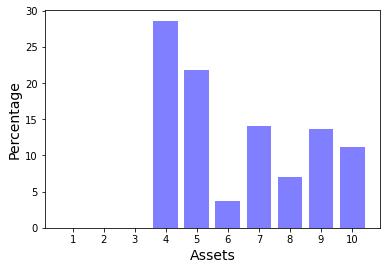
The optimal decision in terms of asset allocation and the objective value are shown below.
import matplotlib.pyplot as plt

xdata = np.arange(1, m+1)
plt.bar(xdata, x.get()*100, color='b', alpha=0.5)
plt.xticks(xdata)
plt.xlabel('Assets', fontsize=14)
plt.ylabel('Percentage', fontsize=14)
plt.show()
print(model.get())
-1.1362073575769465
Distributionally Robust Model
We can also directly implement the distributionally robust model in a more concise and readable manner using the rsome.dro environment, see the code below.
from rsome import dro
from rsome import E
import rsome as rso

model = dro.Model(n)
x = model.dvar(m)
tau = model.dvar()

z = model.rvar(m)
u = model.rvar()
fset = model.ambiguity()
for s in range(n):
    fset[s].suppset(rso.norm(z - zhat[s], 1) <= u, z >= -1)
fset.exptset(E(u) <= epsilon)
pr = model.p
fset.probset(pr == 1/n)

r = z @ x
model.minsup(E(rso.maxof(a1*r + b1*tau,
                         a2*r + b2*tau)), fset)
model.st(x.sum() == 1, x >= 0)

model.solve()
Being solved by the default LP solver...
Solution status: 0
Running time: 0.0814s
Here, we are using the rso.maxof() function to define a piecewise expression of the maximum of two given terms a1*r + b1*tau and a2*r + b2*tau. Solution of this model is exactly the same as the deterministic equivalent problem.
Reference
Mohajerin Esfahani, Peyman, and Daniel Kuhn. 2018. Data-driven distributionally robust optimization using the Wasserstein metric: Performance guarantees and tractable reformulations. Mathematical Programming 171 115-166.
Rockafellar, R. Tyrrell, and Stanislav Uryasev. 2000. Optimization of conditional value-at-risk. Journal of risk 2 21-42.
Chen, Zhi, Melvyn Sim, Peng Xiong. 2020. Robust stochastic optimization made easy with RSOME. Management Science 66(8) 3329–3339.