| Star | Watch | Fork |
| Home |
|---|
| User Guide |
| Examples |
| About |
Minimal Enclosing Ellipsoid
In this example, we consider a polytope given as the convex hull of \(m\) of data points,
\[S = \text{conv}\left\{\pmb{x}_1, \pmb{x}_2, ..., \pmb{x}_m\right\}, ~~~\pmb{x}_i \in \mathbb{R}^n.\]The polytope is enclosed in the following ellipsoid
\[\mathcal{E} := \left\{\pmb{x}\left|\|\pmb{Px} - \pmb{c}\|_2 \leq 1 \right.\right\},\]where \(\pmb{P}\) and \(\pmb{c}\) are the coefficients of the ellipsoid. According to MOSEK Modeling Cookbook, the minimum-volume enclosing ellipsoid can be achieved via solving the solving semidefinite programming problem.
\[\begin{align} \max~&\text{det}(\pmb{P}) \\ \text{s.t.}~&\|\pmb{Px}_i - \pmb{c}\|_2 \leq 1, &i=1, 2, ..., m \\ &\pmb{P} \succeq 0. \end{align}\]The function \(\text{det}(\cdot)\) indicates the determinant of a given matrix, which is either convex or concave, but the logarithm of the determinant is concave, and maximizing \(\log(\text{det}(\pmb{P}))\) is equivalent to the following conic programming problem:
\[\begin{align} \max~&\sum\limits_{i=1}^n v_i \\ \text{s.t.}~&v_i \leq \log(Z_{ii}), &i=1, 2, ..., n\\ &\left( \begin{array}{cc} \pmb{P} & \pmb{Z} \\ \pmb{Z}^{\top} & \text{diag}(\pmb{Z}) \end{array} \right) \succeq 0 \\ &\pmb{Z}\text{ if lower triangular}. \end{align}\]Therefore, the minimum-volume enclosing ellipsoid problem can be rewritten as follows.
\[\begin{align} \max~&\sum\limits_{i=1}^n v_i \\ \text{s.t.}~&v_i \leq \log(Z_{ii}), &i=1, 2, ..., n\\ &\left( \begin{array}{cc} \pmb{P} & \pmb{Z} \\ \pmb{Z}^{\top} & \text{diag}(\pmb{Z}) \end{array} \right) \succeq 0 \\ &\|\pmb{Px}_i - \pmb{c}\|_2 \leq 1, &i=1, 2, ..., m \\ &\pmb{P} \succeq 0 \\ &\pmb{Z}\text{ if lower triangular}. \end{align}\]In the following numerical experiments, the data points are randomly generated with \(n=2\) and \(m=50\) by the code segment below.
import numpy as np
import matplotlib.pyplot as plt

m = 50
np.random.seed(1)
xs = np.random.randn(m, 2)
xs[:, 1] = xs[:, 0]*0.08 + xs[:, 1]
The Python code for implementing the model above is presented below.
from rsome import ro
from rsome import cpt_solver as cpt
import rsome as rso

model = ro.Model()

P = model.dvar((2, 2))
c = model.dvar(2)
Z = rso.tril(model.dvar((2, 2)))
v = model.dvar(2)

model.max(v.sum())
model.st(v <= rso.log(rso.diag(Z)))
model.st(rso.rstack([P, Z],
                    [Z.T, rso.diag(Z, fill=True)]) >> 0)
for i in range(m):
    model.st(rso.norm(P@xs[i] - c) <= 1)
model.st(P >> 0)

model.solve(cpt)
print(f'Determinant: {np.exp(model.get())}')
Being solved by COPT...
Solution status: 1
Running time: 0.0185s
Determinant: 0.23537956658491654
The boundary of the ellipsoid is achieved by the following code using the solution of \(\pmb{P}\) and \(\pmb{c}\).
Ps = P.get()
cs = c.get()

step = 0.01
t = np.arange(0, 2*np.pi+step, step)
y = np.vstack((np.cos(t), np.sin(t))).T

ellip = np.linalg.inv(Ps) @ (y + cs).T
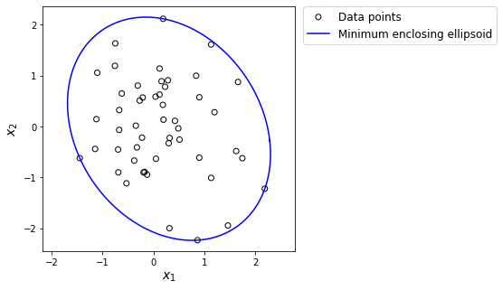
Finally, the enclosing ellipsoid and randomly generated data points are shown below.
plt.figure(figsize=(5, 5))
plt.scatter(xs[:, 0], xs[:, 1],
            marker='o', facecolor='none', color='k', label='Data points')
plt.plot(ellip[0], ellip[1], color='b',
         label='Minimum enclosing ellipsoid')
plt.legend(fontsize=12, bbox_to_anchor=(1.01, 1.02))
plt.axis('equal')
plt.xlabel(r'$x_1$', fontsize=14)
plt.ylabel(r'$x_2$', fontsize=14)
plt.show()