
| Star | Watch | Fork |
| Home |
|---|
| User Guide |
| Examples |
| About |
Distributionally Robust Portfolio under Moment Uncertainty
In this example, we will use RSOME to the solve the portfolio problem discussed in Delage and Ye 2010. The portfolio problem is formulated as the following distributionally robust model,
\[\begin{align} \min~&\sup\limits_{\mathbb{P}\in\mathcal{F}}\mathbb{E}\left[\alpha + \frac{1}{\epsilon}\max\left\{-\tilde{\pmb{\xi}}^{\top}\pmb{x} - \alpha, 0\right\}\right] \\ \text{s.t.}~&\pmb{e}^{\top}\pmb{x}=1, \pmb{x}\in\mathbb{R}_+^{n}. \end{align}\]where \(\tilde{\pmb{\xi}}\in\mathbb{R}^n\) is a random vector representing the uncertain returns of \(n\) stocks, and the objective function minimizes the conditional value-at-risk (CVaR) of the investment return under the worst-case distribution \(\mathbb{P}\) over the ambiguity set \(\mathcal{F}\), defined below
\[\mathcal{F} = \left\{ \mathbb{P}\in\mathcal{P}_0\left(\mathbb{R}^n\right) \left| \begin{array} \tilde{\pmb{\xi}} \sim \mathbb{P} \\ \left(\mathbb{E}[\tilde{\pmb{\xi}}] - \mu\right)^{\top}\Sigma^{-1}\left(\mathbb{E}[\tilde{\pmb{\xi}}] - \mu\right) \leq \gamma_1 \\ \mathbb{E}\left[\left(\tilde{\pmb{\xi}}-\mu\right)\left(\tilde{\pmb{\xi}}-\mu\right)^{\top}\right] \preceq \gamma_2 \Sigma \end{array} \right. \right\}.\]According to Delage and Ye 2010, the distributionally robust model is equivalent to the following convex optimization problem
\[\begin{align} \min~&r + t \\ \text{s.t.}~& \left( \begin{array} \\\pmb{Q} & \pmb{q}/2 + (1/\epsilon)\pmb{x}/2 \\ \pmb{q}^{\top}/2 + (1/\epsilon)\pmb{x}^{\top}/2 & r + (1-\epsilon)/\epsilon\alpha \end{array} \right) \succeq 0\\ &\left( \begin{array} \\\pmb{Q} & \pmb{q}/2 \\ \pmb{q}^{\top}/2 & r - \alpha \end{array} \right) \succeq 0\\ &t \geq (\gamma_2\pmb{\Sigma} + \pmb{\mu}\pmb{\mu}^{\top}) \boldsymbol{\cdot} \pmb{Q} + \pmb{\mu}^{\top}\pmb{q} + \sqrt{\gamma_1}\|\pmb{\Sigma}^{1/2}(\pmb{q} + 2\pmb{Q\mu})\| \\ &\pmb{Q} \succeq 0 \\ &\pmb{e}^{\top}\pmb{x}=1, \pmb{x}\in\mathbb{R}_+^{n}. \end{align}\]In the numerical experiments below, the mean returns \(\pmb{\mu}\) and covariance matrix \(\pmb{\Sigma}\) are estimated using the sample data of eight stocks “JPM”, “AMZN”, “TSLA”, “AAPL”, “GOOG”, “ZM”, “META”, and “MCD”, in the year of 2021.
import pandas as pd
import yfinance as yf

stocks = ['JPM', 'AMZN', 'TSLA', 'AAPL', 'GOOG', 'ZM', 'META', 'MCD']
start = '2021-01-01'
end='2021-12-31'

data = pd.DataFrame([])
for stock in stocks:
    each = yf.Ticker(stock).history(start=start, end=end)
    close = each['Close'].values
    returns = (close[1:] - close[:-1]) / close[:-1]
    data[stock] = returns

data
| JPM | AMZN | TSLA | AAPL | GOOG | ZM | META | MCD | |
|---|---|---|---|---|---|---|---|---|
| 0 | 0.005441 | 0.010004 | 0.007317 | 0.012364 | 0.007337 | 0.002361 | 0.007548 | 0.005994 |
| 1 | 0.046956 | -0.024897 | 0.028390 | -0.033662 | -0.003234 | -0.045506 | -0.028269 | -0.002270 |
| 2 | 0.032839 | 0.007577 | 0.079447 | 0.034123 | 0.029943 | -0.005546 | 0.020622 | 0.004645 |
| 3 | 0.001104 | 0.006496 | 0.078403 | 0.008631 | 0.011168 | 0.020759 | -0.004354 | 0.018351 |
| 4 | 0.014924 | -0.021519 | -0.078214 | -0.023249 | -0.022405 | -0.034038 | -0.040102 | -0.007597 |
| ... | ... | ... | ... | ... | ... | ... | ... | ... |
| 245 | 0.003574 | 0.000184 | 0.057619 | 0.003644 | 0.001317 | -0.007663 | 0.014495 | 0.003812 |
| 246 | 0.005723 | -0.008178 | 0.025248 | 0.022975 | 0.006263 | -0.021967 | 0.032633 | 0.008610 |
| 247 | 0.003035 | 0.005844 | -0.005000 | -0.005767 | -0.010914 | -0.019580 | 0.000116 | -0.001342 |
| 248 | -0.000504 | -0.008555 | -0.002095 | 0.000502 | 0.000386 | -0.010666 | -0.009474 | 0.002277 |
| 249 | -0.000505 | -0.003289 | -0.014592 | -0.006578 | -0.003427 | 0.047907 | 0.004141 | -0.004767 |
250 rows × 8 columns
μ = data.mean().values
Σ = data.cov().values
Parameters \(\gamma_1\) and \(\gamma_2\) in the ambiguity set \(\mathcal{F}\), together with the risk tolerance level \(\epsilon\), are specified in the code segment below.
γ1, γ2 = 0.25, 1.50
ε = 0.05
The equivalent convex optimization problem can be then implemented by the following python code.
from rsome import ro
from rsome import msk_solver as msk
import rsome as rso
from scipy.linalg import sqrtm

model = ro.Model()

n = len(μ)
x = model.dvar(n)
α = model.dvar()
Q = model.dvar((n, n))
q = model.dvar(n)
r = model.dvar()
t = model.dvar()
s = model.dvar()

model.min(r + t)
model.st(t >= γ2*(Σ*Q).sum() + μ@Q@μ + μ@q +
         γ1**0.5*rso.norm(sqrtm(Σ)@(q + 2*Q@μ)))

vec = (q*0.5 + (1/ε)*x*0.5)[None, :]
model.st(rso.rstack([Q, vec.T],
                    [vec, r+(1-ε)/ε*α]) >> 0)

vec = (q*0.5)[None, :]
model.st(rso.rstack([Q, vec.T],
                    [vec, r-α]) >> 0)

model.st(Q >> 0)
model.st(x >= 0, x.sum() == 1)

model.solve(msk)

print(f'Objective value: {model.get():.6f}')
Being solved by Mosek...
Solution status: Optimal
Running time: 0.0199s
Objective value: 0.042948
Note that the ambiguity set \(\mathcal{F}\) can also be written as the following lifted version,
\[\mathcal{G} = \left\{ \mathbb{P}\in\mathcal{P}_0\left(\mathbb{R}^n\times\mathbb{S}^n\right) \left| \begin{array}{l} (\tilde{\pmb{\xi}}, \tilde{\pmb{U}}) \sim \mathbb{P} \\ \mathbb{P}\left[ \left( \begin{array}{ll} \tilde{\pmb{U}} & \tilde{\pmb{\xi}} - \pmb{\mu} \\ \tilde{\pmb{\xi}}^{\top} - \pmb{\mu}^{\top} & 1 \end{array} \right) \succeq 0 \right] = 1 \\ \left(\mathbb{E}[\tilde{\pmb{\xi}}] - \mu\right)^{\top}\Sigma^{-1}\left(\mathbb{E}[\tilde{\pmb{\xi}}] - \mu\right) \leq \gamma_1 \\ \mathbb{E}\left[\tilde{\pmb{U}}\right] = \gamma_2 \Sigma \end{array} \right. \right\},\]where the support of the ambiguity set is used to enforce the constraint \(\left(\tilde{\pmb{\xi}} - \pmb{\mu}\right)\left(\tilde{\pmb{\xi}} - \pmb{\mu}\right)^{\top} \preceq \tilde{\pmb{U}}\). Such an ambiguity set can be directly constructed using the RSOME package, so the distributionally robust optimization model can be implemented in a more concise and readable manner.
from rsome import dro
from rsome import msk_solver as msk
from rsome import E
import rsome as rso
import numpy as np

model = dro.Model()

n = len(μ)
x = model.dvar(n)
α = model.dvar()

ξ = model.rvar(n)
U = model.rvar((n, n))
gset = model.ambiguity()
gset.suppset(rso.rstack([U, (ξ - μ)[:, None]],
                        [(ξ - μ)[None, :], 1]) >> 0)
inv_Σ = np.linalg.inv(Σ)
gset.exptset(rso.quad(E(ξ) - μ, inv_Σ) <= γ1,
             E(U) == γ2*Σ)

model.minsup(α + (1/ε)*E(rso.maxof(-ξ@x - α, 0)), gset)
model.st(x.sum() == 1, x >= 0)

model.solve(msk)

print(f'Objective value: {model.get():.6f}')
Being solved by Mosek...
Solution status: Optimal
Running time: 0.0304s
Objective value: 0.042948
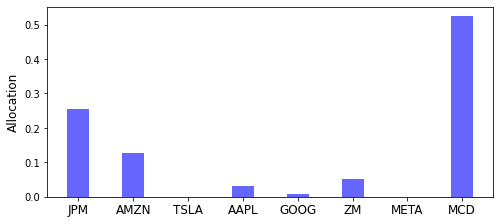
Both convex optimization problems above give the same investment decision, which is visualized by the following code.
import matplotlib.pyplot as plt

plt.figure(figsize=(8, 3.5))
plt.bar(data.columns, x.get(), width=0.4, color='b', alpha=0.6)
plt.xticks(fontsize=12)
plt.ylabel('Allocation', fontsize=12)
plt.show()
Reference
Delage, Erick, and Yinyu Ye. 2010. Distributionally robust optimization under moment uncertainty with application to data-driven problems. Operations Research 58(3) 595-612.