
| Star | Watch | Fork |
| Home |
|---|
| User Guide |
| Examples |
| About |
Mean-Variance Portfolio
In this example, we consider a portfolio optimization problem discussed in Ben-Tal and Nemirovski (1999). Suppose there are \(n=150\) stocks, and each stock \(i\) has the mean return to be \(p_i\) and the standard deviation to be \(\sigma_i\). Let \(x_i\) be the fraction of the total wealth invested in stock \(i\), a classic approach is to formulate the problem as a quadratic program, where a mean-variance objective function is maximized:
\[\begin{align} \max~&\sum\limits_{i=1}^np_ix_i - \phi \sum\limits_{i=1}^n \sigma_i^2x_i^2 \\ \text{s.t.}~&\sum\limits_{i=1}^nx_i = 1 \\ & x_i \geq 0, ~\forall i = 1, 2, ..., n, \end{align}\]with the constant \(\phi=5\), and the means and standard deviations are specified as
\[\begin{align} &p_i = 1.15 + i\frac{0.05}{150} & \forall i = 1, 2, ..., n\\ &\sigma_i = \frac{0.05}{450}\sqrt{2in(n+1)} & \forall i = 1, 2, ..., n. \end{align}\]The quadratic program can be implemented by the following code segment.
from rsome import ro
from rsome import grb_solver as grb
import rsome as rso
import numpy as np

n = 150                                     # number of stocks
i = np.arange(1, n+1)                       # indices of stocks
p = 1.15 + i*0.05/150                       # mean returns
sigma = 0.05/450 * (2*i*n*(n+1))**0.5       # standard deviations of returns
phi = 5                                     # constant phi

model = ro.Model('mv-portfolio')            # create an RSOME model

x = model.dvar(n)                           # fractions of investment

Q = np.diag(sigma**2)                       # covariance matrix
model.max(p@x - phi*rso.quad(x, Q))         # mean-variance objective
model.st(x.sum() == 1)                      # summation of x is one
model.st(x >= 0)                            # x is non-negative

model.solve(grb)
Being solved by Gurobi...
Solution status: 2
Running time: 0.0028s
The optimal investment and the optimal objective value are shown below.
import matplotlib.pyplot as plt

obj_val = model.get()               # the optimal objective value
x_sol = x.get()                     # the optimal investment decision

plt.plot(range(1, n+1), x_sol,
         linewidth=2, color='b')
plt.xlabel('Stocks')
plt.ylabel('Fraction of investment')
plt.show()
print('Objective value: {0:0.4f}'.format(obj_val))
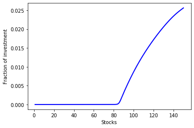
Objective value: 1.1853
Reference
Ben-Tal, Aharon, and Arkadi Nemirovski. 1999. Robust solutions of uncertain linear programs. Operations Research Letters 25(1) 1-13.