Robust Stochastic Optimization Made Easy by XiongPengNUS

Home
User Guide
Examples
About

Robust/Robustness Knapsack

In this example, we will use the RSOME package to implement the robust knapsack model introduced in the paper Bertsimas and Sim (2004), and the robustness model described in the paper Long et al. (2019). In the knapsack problem, the weight coefficient \(\tilde{w}_i\) is assumed to be randomly distributed in the range \([w_i - \delta_i, ~ w_i + \delta_i]\). Suppose that each good has a value of \(c_i\), then the objective is to maximize the total value of goods. The robust model can be thus written as

\[\begin{align} \max~&\sum\limits_{i=1}^nc_i x_i \\ \text{s.t.}~&\sum\limits_{i=1}^n({w}_i + z_i\delta_i)x_i \leq b, \forall \pmb{z} \in \mathcal{Z} \\ &\pmb{x} \in \{0, 1\}^n \end{align}\]

with the array \(\pmb{z}\) representing random variables, which are constrained by an uncertainty set

\[\begin{align} \mathcal{Z}=\left\{\pmb{z}: \|\pmb{z}\|_{\infty} \leq 1, \|\pmb{z}\|_{1} \leq r\right\}. \end{align}\]

The parameter \(r\) is the budget of uncertainty. The robustness optimization model can be formulated by introducing auxiliary random variables \(\pmb{u}\), such that

\[\begin{align} \min~&k\\ \text{s.t.}~&\sum\limits_{i=1}^nc_i x_i \geq \tau \\ &\sum\limits_{i=1}^n({w}_i + z_i\delta_i)x_i - b \leq k \sum\limits_{i=1}^nu_i, \forall (\pmb{z}, \pmb{u}) \in \overline{\mathcal{Z}} \\ &\pmb{x} \in \{0, 1\}^n \end{align}\]

with \(\tau\) to a target of the objective value, and the random variables \(\pmb{z}\) and \(\pmb{u}\) constrained by an lifted uncertainty set \(\begin{align} \overline{\mathcal{Z}}=\left\{(\pmb{z}, \pmb{u}): |z_i|\leq u_i\leq 1, \forall i=1, 2, ..., n \right\}. \end{align}\)

Following the aforementioned papers, parameters \(\pmb{c}\), \({\pmb{w}}\), and \(\pmb{\delta}\) are randomly generated by the code below.

from rsome import ro
from rsome import grb_solver as grb
import rsome as rso
import numpy as np
import numpy.random as rd
import matplotlib.pyplot as plt

N = 50
b = 2000

c = 2*rd.randint(low=5, high=10, size=N)    # profit coefficients
w = 2*rd.randint(low=10, high=41, size=N)   # nominal weights
delta = 0.2*w                               # maximum deviations

The robust optimization model for a given budget of uncertainty \(r\) is written as a function named robust().

def robust(r):
    """
    The function robust implements the robust optimiztion model,
    given the budget of uncertainty r
    """

    model = ro.Model('robust')
    x = model.dvar(N, vtype='B')    
    z = model.rvar(N)              

    z_set = (abs(z) <= 1, rso.norm(z, 1) <= r)
    model.max(c @ x)
    model.st(((w + z*delta) @ x <= b).forall(z_set))

    model.solve(grb, display=False) # disable solution message

    return model.get(), x.get()     # the optimal objective and solution

Similarly, the robustness optimization model for a given target of profit \(\tau\) can also be written as a function robustness().

def robustness(tau):
    """
    The function robustness implements the robustness optimization
    model, given the profit target tau.
    """

    model = ro.Model('robustness')

    x = model.dvar(N, vtype='B')    
    k = model.dvar()              
    z = model.rvar(N)           
    u = model.rvar(N)           

    z_set = (abs(z) <= u, u <= 1)
    model.min(k)
    model.st(c @ x >= tau)
    model.st(((w + z*delta) @ x - b <= k*u.sum()).forall(z_set))
    model.st(k >= 0)

    model.solve(grb, display=False) # disable solution message

    return model.get(), x.get()     # the optimal objective and solution

Given a decision \(\pmb{x}\) and a sample of the random variable \(\pmb{z}\), we write a function sim() to calculate the probability of constraint violation, as an indicator of the performance of solutions.

def sim(x_sol, zs):
    """
    The function sim is for calculating the probability of violation
    via simulations.
        x_sol: solution of the Knapsack problem
        zs: random sample of the random variable z
    """

    ws = w + zs*delta   # random samples of uncertain weights

    return (ws @ x_sol > b).mean()

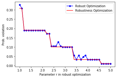
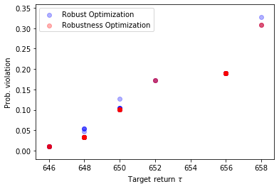
According to Long et al. (2019), the robust models are solved first under different budgets of uncertainty. The corresponding objective values are then used as total value targets in the robustness optimization models. Solutions of the robust and robustness models are assessed via simulation to find out the probabilities of violations.

step = 0.1
rs = np.arange(1, 5+step, step)         # all budgets of uncertainty
num_samp = 20000
zs = 1-2*rd.rand(num_samp, N)           # random samples for z

"""Robust optimization"""
outputs_rb = [robust(r) for r in rs]
targets = [output[0]
           for output in outputs_rb]    # RO objective as targets
pv_rb = [sim(output[1], zs)
         for output in outputs_rb]      # probability of violations

"""Robustness optimization"""
outputs_rbn = [robustness(target)
               for target in targets]   
pv_rbn = [sim(output[1], zs)
          for output in outputs_rbn]    # probability of violations

Finally, the probabilities of violations for both methods are visualized by the following diagrams.

plt.plot(rs, pv_rb, marker='o', markersize=5, c='b',
         label='Robust Optimization')
plt.plot(rs, pv_rbn, c='r',
         label='Robustness Optimization')

plt.legend()
plt.xlabel('Parameter r in robust optimization')
plt.ylabel('Prob. violation')
plt.show()

plt.scatter(targets, pv_rb, c='b', alpha=0.3,
            label='Robust Optimization')
plt.scatter(targets, pv_rbn, c='r', alpha=0.3,
            label='Robustness Optimization')

plt.legend()
plt.xlabel(r'Target return $\tau$')
plt.ylabel('Prob. violation')
plt.show()

png

Reference

Bertsimas, Dimitris, and Melvyn Sim. 2004. The price of robustness. Operations Research 52(1) 35-53.

Long, Daniel Zhuoyu, Melvyn Sim, and Minglong Zhou. 2019. The dao of robustness.