Robust Stochastic Optimization Made Easy by XiongPengNUS

Home
User Guide
Examples
About

The Unit Commitment Problem

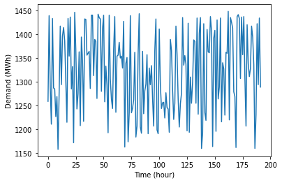
In this example, we attempt to solve a unit commitment (UC) problem described in the tutorial of IBM Decision Optimization CPLEX for Python (DOcplex). The electricity demand data and parameters of all generators are read from the data file uc_data.xlsx, by code segments below.

import pandas as pd
import matplotlib.pyplot as plt

demand = pd.read_excel('uc_data.xlsx', 'Demand')     # Electricity demand 
plt.plot(demand.index, demand['load'])
plt.xlabel('Time (hour)')
plt.ylabel('Demand (MWh)')
plt.show()

units = pd.read_excel('uc_data.xlsx', 'Units')       # Parameters of generators
units

	name	energy	initial	min_gen	...	start_cost	fixed_cost	variable_cost	co2_cost
0	coal1	coal	400	100.00	...	5000	208.610	22.536	30
1	coal2	coal	350	140.00	...	4550	117.370	31.985	30
2	gas1	gas	205	78.00	...	1320	174.120	70.500	5
3	gas2	gas	52	52.00	...	1291	172.750	69.000	5
4	gas3	gas	155	54.25	...	1280	95.353	32.146	5
5	gas4	gas	150	39.00	...	1105	144.520	54.840	5
6	diesel1	diesel	78	17.40	...	560	54.417	40.222	15
7	diesel2	diesel	76	15.20	...	554	54.551	40.522	15
8	diesel3	diesel	0	4.00	...	300	79.638	116.330	15
9	diesel4	diesel	0	2.40	...	250	16.259	76.642	15

10 rows × 14 columns

Parameters of the UC model are specified by the code segment below,

g_init = units['initial'].values
u_init = (g_init > 0).astype(int)
g_min = units['min_gen'].values
g_max = units['max_gen'].values
h_up = units['min_uptime'].values
h_down = units['min_downtime'].values
r_up = units['ramp_up'].values
r_down = units['ramp_down'].values
a = units['fixed_cost'].values
b = units['variable_cost'].values
c = units['start_cost'].values
d = demand['load'].values
e = units['co2_cost'].values

and detailed information on these parameters is provided in the following table.

Notation	Interpretation	Array Expression	Python Variable
\(g_n^{\text{init}}\)	The initial output of the \(n\)th generator	`units['initial'].values`	`g_init`
\(u_n^{\text{init}}\)	The initial on/off status of the \(n\)th generator	`(g_init > 0).astype(int)`	`u_init`
\(g_n^{\text{min}}\)	The minimum capacity of the \(n\)th generator	`units['min_gen'].values`	`g_min`
\(g_n^{\text{max}}\)	The maximum capacity of the \(n\)th generator	`units['max_gen'].values`	`g_max`
\(h_n^{\text{up}}\)	The minimum up time of the \(n\)th generator	`units['min_uptime'].values`	`h_up`
\(h_n^{\text{down}}\)	The minimum down time of the \(n\)th generator	`units['min_downtime'].values`	`h_down`
\(r_n^{\text{up}}\)	The ramp-up rate limit of the \(n\)th generator	`units['ramp_up'].values`	`r_up`
\(r_n^{\text{down}}\)	The ramp-down rate limit of the \(n\)th generator	`units['ramp_down'].values`	`r_down`
\(a_n\)	The fixed cost of the \(n\)th generator	`units['fixed_cost'].values`	`a`
\(b_n\)	The variable cost of the \(n\)th generator	`units['variable_cost'].values`	`b`
\(c_n\)	The start-up cost of the \(n\)th generator	`units['start_cost'].values`	`c`
\(d_t\)	The demand at time step \(t\)	`demand['load'].values`	`d`
\(e_t\)	The CO2 emission cost of the \(n\)th generator	`units['co2_cost'].values`	`e`

The UC model that determines the on/off statues of generators and their outputs in supplying the electricity demand can be written as the following mixed-integer linear programming problem.

\[\begin{align} \min~&\sum\limits_{t=1}^T\sum\limits_{n=1}^N\left(a_nu_{tn} + b_ng_{tn} + c_nv_{tn} + e_ng_{tn}\right) \hspace{-1in}& \\ \text{s.t.}~&v_{1n} \geq u_{1n} - u_n^{\text{init}}, v_{1n} \geq 0 &\forall n= 1, ..., N \\ &v_{tn} \geq u_{tn} - u_{(t-1)u}, v_{tn} \geq 0 & \forall t = 2, ..., T, \forall n = 1, ..., N \\ &w_{1n} \geq u_n^{\text{init}} - u_{1n}, w_{1n} \geq 0 &\forall n= 1, ..., N \\ &w_{tn} \geq u_{(t-1)u} - u_{tn}, w_{tn} \geq 0 & \forall t = 2, ..., T, \forall n = 1, ..., N \\ &\sum\limits_{k=t-h_n^{\text{up}}+1}^tv_{tn} \leq u_{tn} & \forall t=h_n^{\text{up}}, ..., T, \forall n = 1, ..., N \\ &\sum\limits_{k=t-h_n^{\text{down}}+1}^tw_{tn} \leq 1 - u_{tn} & \forall t=h_n^{\text{down}}, ..., T, \forall n = 1, ..., N \\ &\sum\limits_{n=1}^Tg_{tn} = d_{t} &\forall t=1, ..., T \\ &u_{tn}g_n^{\text{min}} \leq g_{tn} \leq u_{tn}g_n^{\text{max}} &\forall t=1, ..., T, \forall n = 1, ..., N \\ &g_{1n} - g_n^{\text{init}} \leq r_n^{\text{up}} &\forall n = 1, ..., N \\ &g_{tn} - g_{(t-1)n} \leq r_n^{\text{up}} &\forall t=2, ..., T, \forall n=1, ..., N \\ &g_n^{\text{init}} - g_{1n} \leq r_n^{\text{down}} &\forall n = 1, ..., N \\ &g_{(t-1)n} - g_{tn} \leq r_n^{\text{down}} &\forall t=2, ..., T, \forall n=1, ..., N \end{align}\]

where \(T\) is the number of time steps, and \(N\) is the number of generator units. The decision variables are explained in the following table.

Notation	Interpretation	Python Variable
\(u_{tn}\)	Binary variable indicating the status of the \(n\)th generator at time \(t\)	`u`
\(v_{tn}\)	Binary variable indicating if the \(n\)th generator is switched on at time \(t\)	`v`
\(w_{tn}\)	Binary variable indicating if the \(n\)th generator is switched off at time \(t\)	`w`
\(g_{tn}\)	Continuous variable representing the output of the \(n\)th generator at time \(t\)	`g`

The UC model above can be implemented by the following Python code.

from rsome import ro

model = ro.Model('UC')                           # Create a model named 'UC'

N = units.shape[0]                               # Number of units
T = len(d)                                       # Number of time steps
u = model.dvar((T, N), 'B')                      # Unit commitment statuses
v = model.dvar((T, N), 'B')                      # Switch-on statuses of units
w = model.dvar((T, N), 'B')                      # Switch-off statuses of units
g = model.dvar((T, N))                           # Generation outputs

model.min((a*u + b*g + c*v + e*g).sum())         # Minimize the total cost
model.st(v[0] >= u[0] - u_init, 
         v[1:] >= u[1:] - u[:-1],
         v >= 0)                                 # Switch-on statuses
model.st(w[0] >=  u_init - u[0], 
         w[1:] >= u[:-1] - u[1:],
         w >= 0)                                 # Switch-off statuses                
for n in range(N):
    model.st(v[t-h_up[n]+1:t+1, n].sum() <= u[t, n] 
             for t in range(h_up[n], T))         # Minimum up time constraints
    model.st(w[t-h_down[n]+1:t+1, n].sum() <= 1 - u[t, n]
             for t in range(h_down[n], T))       # Minimum down time constraints
model.st(g.sum(axis=1) == d)                     # Power balance equation
model.st(g >= u*g_min,                           # Minimum capacities of units
         g <= u*g_max)                           # Maximum capacities of units
model.st(g[1:] - g[:-1] <= r_up,
         g[0] - g_init <= r_up,                  # Ramp-up rate limits
         g[:-1] - g[1:] <= r_down,
         g_init - g[0] <= r_down)                # Ramp-down rate limits

model.solve()                                    # Solve the model

print(f'\nMinimum cost: {model.get():.4f}')

Being solved by the default MILP solver...
Solution status: 0
Running time: 1.4817s

Minimum cost: 14213082.0639

Please note that here we are using the default solver imported from the scipy.optimize to solve the mixed-integer linear programming problem. The default solver is able to address integer variables only if the version of the installed SciPy package is 1.9.0 or above. For SciPy 1.8.1 or older version, the default solver is unable to include integrality constraints, so the problem can only be solved by the updated SciPy solver or other solvers.

Similar to the case study discussed in the unit commitment (UC) problem, each component of the operating cost is calculated and listed below.

print(f'Total fixed cost:    {(a * u.get()).sum():.3f}')
print(f'Total variable cost: {(b * g.get()).sum():.3f}')
print(f'Total start-up cost: {(c * v.get()).sum():.3f}')
print(f'Total economic cost: {(a*u.get() + b*g.get() + c*v.get()).sum():.3f}')
print(f'Total CO2 cost:      {(e * g.get()).sum():.3f}')

Total fixed cost:    161025.131
Total variable cost: 8865900.433
Total start-up cost: 2832.000
Total economic cost: 9029757.564
Total CO2 cost:      5183324.500