
| Star | Watch | Fork |
| Home |
|---|
| User Guide |
| Examples |
| About |
Distributionally Robust Vehicle Pre-Allocation
Here, we consider the vehicle pre-allocation problem introduced in Hao et al. (2020). Please refer to Robust Vehicle Pre-Allocation for the detailed problem description and parameters. Such a vehicle pre-allocation problem can be formulated as the following distributionally robust optimization model:
\[\begin{align} \min~&\sum\limits_{i\in[I]}\sum\limits_{j\in[J]}(c_{ij} - r_j)x_{ij} + \sup\limits_{\mathbb{P}\in\mathcal{F}}\mathbb{E}_{\mathbb{P}}\left[\sum\limits_{j\in[J]}r_jy_j(\tilde{s}, \tilde{\pmb{z}})\right] \hspace{-1.5in}&& \\ \text{s.t.}~&y_j(s, \pmb{z}) \geq \sum\limits_{i\in[I]}x_{ij} - d_j && \forall \pmb{z} \in \mathcal{Z}_s, \forall s \in [S], \forall j \in [J] \\ &y_j(s, \pmb{z}) \geq 0 && \forall \pmb{z} \in \mathcal{Z}_s, \forall s \in [S], \forall j \in [J] \\ &y_j \in \overline{\mathcal{A}}(\mathcal{C}, \mathcal{J}) && \forall j \in [J] \\ &\sum\limits_{j\in[J]}x_{ij} \leq q_i && \forall i \in [I] \\ &x_{ij} \geq 0 &&\forall i \in[I], \forall j \in [J], \\ \end{align}\]where \(\tilde{\pmb{z}}\) is a vector of all random variables, including the random demand \(\tilde{\pmb{d}}\) and possible auxiliary random variables, and its distribution is characterized by an event-wise ambiguity set \(\mathcal{F}\). The RSOME dro module provides modeling tools specifically designed for dealing with such event-wise ambiguity sets and the associated event-wise recourse adaptation \(\overline{\mathcal{A}}(\mathcal{C}, \mathcal{J})\), as demonstrated by implementation of the following two data-driven approaches.
Sample Robust Model Using the dro Framework
In addition to implementing the sample robust models using the ro framework (Robust Vehicle Pre-Allocation), Chen et. al (2020) points out that the sample robust model can also be cast into a distributionally robust optimization where the ambiguity set is written as
where the random variable vector \(\tilde{\pmb{z}}=\tilde{\pmb{d}}\), and for each sample \(s\in[S]\), the weight is \(w_s=1/S\) and the corresponding support (uncertainty set) is defined as \(\mathcal{Z}_s=\left\{\pmb{d} \in \left[\underline{\pmb{d}}, \bar{\pmb{d}}\right] \left\vert \left\|\pmb{d} - \hat{\pmb{d}}_s \right\| \leq \varepsilon \right. \right\}\), an \(\varepsilon\)-neighborhood around the sample data point \(\hat{\pmb{d}}\). The multiple-policy approximation mentioned in Bertsimas et. al (2021) suggests that each \(y_j\) affinely depends on the demand realization \(\pmb{d}\) and the affine dependency is different for each sample record, so it can be captured by the event-wise adaptation where \(\mathcal{C}=\{\{1\}, \{2\}, \dots, \{S\}\}\) and \(\mathcal{J}=[J]\).
The same dataset file taxi_rain.csv is used in this example.
import pandas as pd

data = pd.read_csv('https://xiongpengnus.github.io/rsome/taxi_rain.csv')

demand = data.loc[:, 'Region1':'Region10']      # taxi demand data

d_ub = demand.max().values                      # upper bound of demand
d_lb = demand.min().values                      # lower bound of demand
The sample robust model cast into a distributionally robust optimization problem is implemented as follows.
from rsome import dro                               # import the dro module
from rsome import norm                              # import the norm function
from rsome import E                                 # import the expectation notion
from rsome import grb_solver as grb                 # import the Gurobi interface

dhat = demand.values                                # sample demand as an array
S = dhat.shape[0]                                   # sample size of the dataset
epsilon = 0.25                                      # parameter of robustness
w = 1/S                                             # weights of scenarios

model = dro.Model(S)                                # a DRO model with S scenarios

d = model.rvar(J)                                   # random variable d
fset = model.ambiguity()                            # create an ambiguity set
for s in range(S):                                  # for each scenario
    fset[s].suppset(d <= d_ub, d >= d_lb,
                    norm(d - dhat[s]) <= epsilon)   # define the support set
pr = model.p                                        # an array of scenario weights
fset.probset(pr == w)                               # specify scenario weights

x = model.dvar((I, J))                              # here-and-now decision x
y = model.dvar(J)                                   # wait-and-see decision y
y.adapt(d)                                          # y affinely adapts to d
for s in range(S):
    y.adapt(s)                                      # y adapts to each scenario s

model.minsup(((c-r)*x).sum() + E(r@y), fset)        # the worst-case expectation
model.st(y >= x.sum(axis=0) - d, y >= 0)            # robust constraints
model.st(x.sum(axis=1) <= q, x >= 0)                # deterministic constraints

model.solve(grb)                                    # solve the model by Gruobi
Being solved by Gurobi...
Solution status: 2
Running time: 1.1454s
Recall the ro framework in Robust Vehicle Pre-Allocation, the decision rules \((y_{sj}(\pmb{d}))_{s \in [S], j \in [J]}\) therein is defined as a two-dimensional array for devising the multiple-policy approximation. In the the dro framework, \(\pmb{y}\) is defined to be one-dimensional and the multiple-policy adaptation is defined by a loop where the affine adaptation for each sample is automatically created by calling the adapt() method, with s being the sample index.
Moments and Uncertain Covariates
In the works of Hao et. al, the ambiguity set \(\mathcal{F}\) is constructed to consider the conditional means \(\pmb{\mu}_s\) and variances \(\pmb{\phi}_s\), for \(S\) scenario,
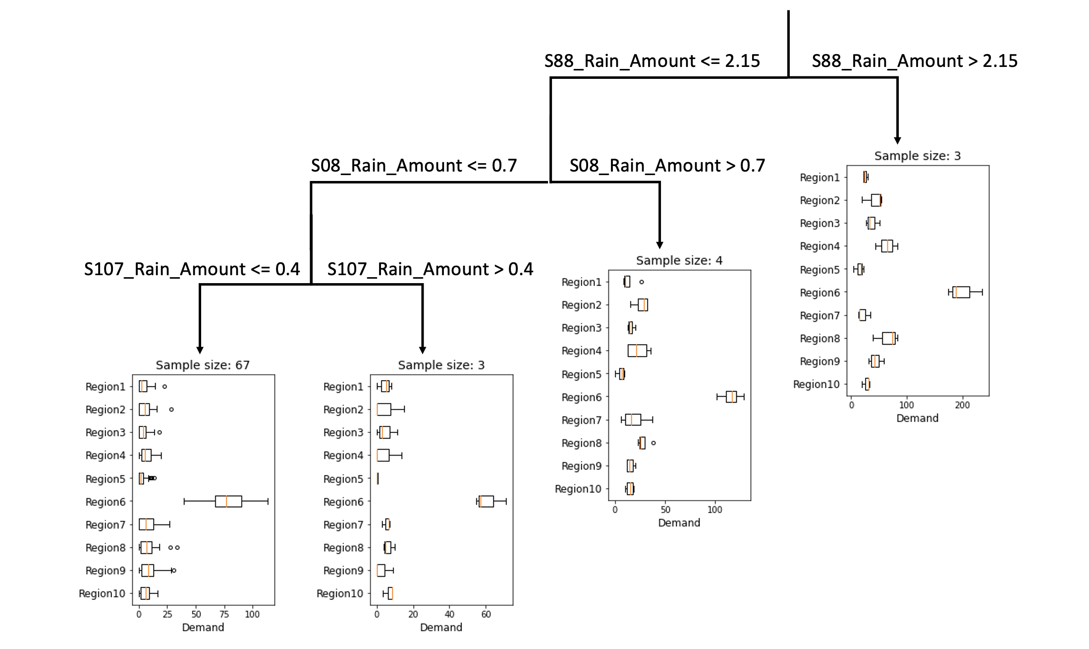
\[\begin{align} \mathcal{F} = \left\{ \mathbb{P}\in\mathcal{P}_0(\mathbb{R}^J\times\mathbb{R}^J\times [S]) \left| \begin{array}{ll} (\tilde{\pmb{d}}, \tilde{\pmb{u}}, \tilde{s}) \in \mathbb{P} & \\ \mathbb{E}_{\mathbb{P}}[\tilde{\pmb{d}}|\tilde{s}=s] = \pmb{\mu}_s & \forall s \in [S] \\ \mathbb{E}_{\mathbb{P}}[\tilde{\pmb{u}}|\tilde{s}=s] = \pmb{\phi}_s & \forall s \in [S] \\ \mathbb{P}[(\tilde{\pmb{d}}, \tilde{\pmb{u}}) \in \mathcal{Z}_s | \tilde{s}=s] = 1 & \forall s \in [S] \\ \mathbb{P}[\tilde{s}=s] = w_s & \forall s \in [S] \\ \end{array} \right. \right\}. \end{align}\]where \(\mathcal{Z}_s=\left\{(\pmb{d},\pmb{u}) \in \mathbb{R}^J \times \mathbb{R}^J: \pmb{d} \in \left[\underline{\pmb{d}}_s, \overline{\pmb{d}}_s\right], ~ (d_j - \mu_j)^2 \leq u_j, ~\forall j \in [J]\right\}\) is the lifted support for each scenario \(s\), and the vector of all random variables is \(\tilde{\pmb{z}} = \left(\tilde{\pmb{d}}, \tilde{\pmb{u}}\right)\). The vector \(\pmb{w}\) is used to denote scenario weights, which amount to the fractions of data points residing in each scenario. Scenarios of the ambiguity set are generated from the dataset taxi_rain.csv, where the first ten columns are the taxi demand data for ten regions, and the remaining columns are corresponding side information in terms of rainfall records, using a decision tree regressor. Assuming the maximum lead node number is four, and the minimum sample size of each leaf is three, then the code for generating scenarios and calculating parameters \(\tilde{\pmb{\mu}}\), \(\tilde{\pmb{\phi}}\), \(\overline{\pmb{d}}\), \(\underline{\pmb{d}}\) and \(\pmb{w}\) (i.e., mu, phi, d\_ub, d\_lb, and w in the code segment, respectively) is given as follows.
from sklearn.tree import DecisionTreeRegressor
import pandas as pd

data = pd.read_csv('https://xiongpengnus.github.io/rsome/taxi_rain.csv')

D, V = data.iloc[:, :10], data.iloc[:, 10:]         # D: demand & V: side information

S = 4
regr = DecisionTreeRegressor(max_leaf_nodes=S,      # max leaf nodes
                             min_samples_leaf=3)    # min sample size of each leaf
regr.fit(V, D)
mu, index, counts = np.unique(regr.predict(V), axis=0,
                              return_inverse=True,
                              return_counts=True)   # mu as the conditional mean
w = counts/V.shape[0]                               # scenario weights
phi = np.array([D.values[index==i].var(axis=0)
                for i in range(len(counts))])       # conditional variance
d_ub = np.array([D.values[index==i].max(axis=0)
                 for i in range(len(counts))])      # upper bound of each scenario
d_lb = np.array([D.values[index==i].min(axis=0)
                 for i in range(len(counts))])      # lower bound of each scenario
The structure of the tree is displayed by the following diagram, as an example of four leaf nodes where the minimum sample size for each node is three.
The event-wise affine adaptation is specified as \(\mathcal{J} = [2J]\) and \(\mathcal{C} = \{\{1\}, \{2\}, \dots, \{S\}\}\), implying that each recourse decision \(y_j\) affinely adapts to random variables \((\tilde{\pmb{d}}, \tilde{\pmb{u}})\) and the affine adaptation may vary in each scenario. The distributionally robust model is implemented by the code below.
from rsome import dro                         # import the dro module
from rsome import square                      # import the element-wise square function
from rsome import E                           # import the notion of expectation
from rsome import grb_solver as grb           # import the solver interface for Gurobi

model = dro.Model(S)                          # create a DRO model with S scenarios

d = model.rvar(J)                             # random demand as the variable d
u = model.rvar(J)                             # auxiliary random variable u
fset = model.ambiguity()                      # create an ambiguity set
for s in range(S):                            # for each scenario:
    fset[s].exptset(E(d) == mu[s],            # specify the expectation set of d and u
                    E(u) <= phi[s])
    fset[s].suppset(d >= d_lb[s],             # specify the support of d and u
                    d <= d_ub[s],
                    square(d - mu[s]) <= u)
pr = model.p                                  # an array of scenario probabilities
fset.probset(pr == w)                         # w as scenario weights

x = model.dvar((I, J))                        # here-and-now decision x
y = model.dvar(J)                             # wait-and-see decision y
y.adapt(d)                                    # y affinely adapts to d
y.adapt(u)                                    # y affinely adapts to u
for s in range(S):                            # for each scenario:
    y.adapt(s)                                # affine adaptation of y is different

model.minsup(((c-r)*x).sum() + E(r@y), fset)  # minimize the worst-case expectation
model.st(y >= x.sum(axis=0) - d, y >= 0)      # robust constraints
model.st(x >= 0, x.sum(axis=0) <= q)          # deterministic constraints

model.solve(grb)                              # solve the model by Gurobi
Being solved by Gurobi...
Solution status: 2
Running time: 0.1342s
Reference
Bertsimas, Dimitris, Shimrit Shtern, and Bradley Sturt. 2021. Two-stage sample robust optimization. Operations Research.
Chen, Zhi, Melvyn Sim, Peng Xiong. 2020. Robust stochastic optimization made easy with RSOME. Management Science 66(8) 3329–3339.
Hao, Zhaowei, Long He, Zhenyu Hu, and Jun Jiang. 2020. Robust vehicle pre‐allocation with uncertain covariates. Production and Operations Management 29(4) 955-972.